How Elasticsearch Really Works: A Look Under the Hood

Elasticsearch powers search at companies like Netflix, GitHub, and Uber. But most developers treat it like a black box. You throw documents in, queries come back, and somehow it just works.

I spent time digging into the internals while building a location-based search system. Here's what I learned about how it actually works.

The Inverted Index: The Core Trick

The main trick is simple but clever. Instead of searching through every document (which would be slow), Elasticsearch builds an "inverted index" when you add documents.

Think of it like a book index. Instead of reading every page to find where "Ruby" appears, you flip to the back and see "Ruby: pages 5, 12, 89". That's much faster.

When you add a document with text "Rust is fast", Elasticsearch:

1. Breaks it into words: ["rust", "is", "fast"]
2. Adds to its index: "rust" → document #1, "fast" → document #1
3. Saves extra info like where in the document each word appears

Now when you search for "rust", it just looks up the index. Instant results.

// Simplified view of an inverted index
{
  "rust": [1, 5, 23],
  "fast": [1, 8],
  "programming": [5, 8, 12, 23],
  "language": [5, 12]
}

Search for "rust programming" and Elasticsearch finds documents that appear in both lists. Document #5 and #23 match both terms.

Text Analysis: The Hidden Hero

Before anything gets indexed, text goes through an analyzer. This step matters more than most people realize.

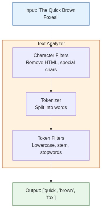
An analyzer does three things:

1. Character filters: Clean up raw text (remove HTML, handle special chars)
2. Tokenizer: Split text into individual tokens (words)
3. Token filters: Modify tokens (lowercase, remove stopwords, stem words)

Both your documents AND search queries go through this same process. That's why "Brown" matches "brown" and "foxes" can match "fox" (with the right analyzer).

// Example: "The Quick Brown Foxes" becomes:
// After standard analyzer:
["the", "quick", "brown", "foxes"]

// After english analyzer (with stemming):
["quick", "brown", "fox"]

This caused me real headaches once. Our location search couldn't find "Starbucks Coffee" when users searched "starbucks café". The problem? Our analyzer didn't handle these variations:

• Convert to lowercase ("Starbucks" → "starbucks")
• Handle synonyms (café, coffee, coffeehouse)
• Remove common words like "the", "is" (optional)
• Handle plurals and word endings

Once we configured the analyzer properly, "coffee shop", "café", and "coffeehouse" all found the same places.

Why Some Results Come First: BM25 Scoring

Elasticsearch uses BM25 scoring to rank results. The algorithm considers three factors:

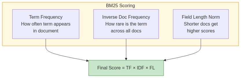
Term frequency (TF): If a word appears many times in a document, it scores higher. A document mentioning "elasticsearch" 10 times is probably more relevant than one mentioning it once.

Inverse document frequency (IDF): Rare words matter more. "Elasticsearch" is more meaningful than "the". IDF measures how rare a term is across all documents.

Field length: Short documents get a boost over long ones for the same match. A 100-word article entirely about Elasticsearch probably beats a 10,000-word article that mentions it twice.

score = TF * IDF * fieldLengthNorm

This is why when you search "rust programming", a short blog post about Rust might rank higher than a long article that mentions Rust once buried in paragraph 47.

Segments and Shards: How It Scales

Elasticsearch doesn't keep everything in one giant index. It splits data into manageable pieces.

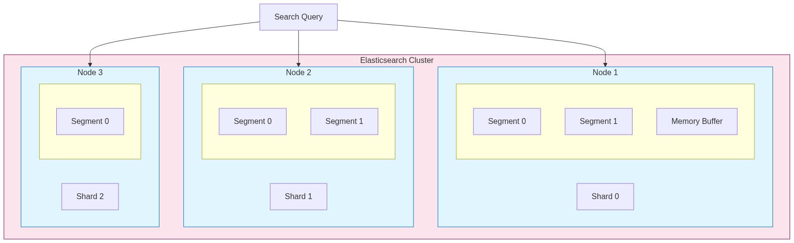
Shards split your index across machines. A 100GB index with 5 shards means each machine handles roughly 20GB. Queries run on all shards in parallel, then results merge together.

Segments are immutable chunks of data within each shard. When you index documents, they first go to an in-memory buffer. Periodically, that buffer gets written to disk as a new segment.

Index
├── Shard 0
│   ├── Segment 0 (immutable)
│   ├── Segment 1 (immutable)
│   └── Memory buffer (new docs)
├── Shard 1
│   ├── Segment 0
│   └── Segment 1
└── Shard 2
    └── ...

Segments are immutable for performance. Instead of updating existing data, Elasticsearch writes new segments and marks old documents as deleted. Background processes merge smaller segments into larger ones over time.

This architecture explains some Elasticsearch quirks:

• Newly indexed documents aren't immediately searchable (they're in the buffer)
• Deletes don't free disk space immediately (just marks documents)
• More segments = slower searches (more places to look)

Real World Example: Location Search

We built a "companies near you" feature searching through 2 million businesses. Users searched "coffee shops in Berlin" and we needed to show the closest ones.

The challenge: combine text search with distance calculations.

We stored each company with:

{
  "name": "Berlin Coffee House",
  "description": "Specialty coffee and pastries in Kreuzberg",
  "location": {
    "lat": 52.4934,
    "lon": 13.4234
  },
  "categories": ["coffee", "cafe", "bakery"]
}

The query combined multiple factors:

{
  "query": {
    "bool": {
      "must": {
        "multi_match": {
          "query": "coffee",
          "fields": ["name^3", "description", "categories^2"]
        }
      },
      "filter": {
        "geo_distance": {
          "distance": "25km",
          "location": {
            "lat": 52.52,
            "lon": 13.405
          }
        }
      }
    }
  },
  "sort": [
    { "_score": "desc" },
    {
      "_geo_distance": {
        "location": { "lat": 52.52, "lon": 13.405 },
        "order": "asc"
      }
    }
  ]
}

The ^3 and ^2 boost matches in specific fields. A match in the name matters more than a match in the description.

The tricky part was balancing distance vs relevance. A perfect name match 10 miles away might be better than a vague match 1 mile away. We tuned the scoring weights until it felt right.

Result: complex location searches returned in under 150ms across 2 million documents.

The Complete Search Flow

Here's what happens when you search:

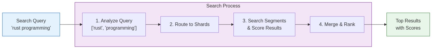
1. Query parsing: Your search text goes through the same analyzer as indexed documents
2. Shard routing: Query goes to all shards (or specific ones if you're clever)
3. Per-shard search: Each shard searches its segments, scores results
4. Coordination: Results from all shards merge and re-rank
5. Return: Top N results come back with scores and highlights

All of this happens in milliseconds.

Practical Takeaways

Choose analyzers carefully. The default standard analyzer works for most cases. Switch to language-specific analyzers (english, german) when you need stemming. Custom analyzers when you have domain-specific requirements.

Understand your shard count. Too few shards limits parallelism. Too many creates overhead. Rule of thumb: aim for shards between 10-50GB each.

Use filters for exact matches. Filters don't calculate scores and get cached. Use them for categories, date ranges, geo boundaries. Save full-text search for when you need ranking.

Watch segment counts. Lots of small segments slow down searches. Force merge during off-peak hours if needed.

# Check segment count
GET /my-index/_segments

# Force merge (use carefully)
POST /my-index/_forcemerge?max_num_segments=1

The Bottom Line

Elasticsearch works through smart organization:

1. Pre-processes everything into an inverted index (like a phone book)
2. Distributes data across shards and segments for scale
3. Uses BM25 to know which words matter for ranking
4. Handles text variations through analyzers so users find what they want

Understanding these internals has helped me build better search systems and debug problems faster. When searches return unexpected results, I now know where to look: analyzer configuration, scoring weights, or shard distribution.

It's not magic. It's good engineering.